The world of ray-tracing, known for its ability to generate photorealistic images, is now at our doorstep. It's there, waiting for real-time 3D engineers to fully understand its potential. In this series of articles, I'll describe my journey of integrating this powerful new tool into my existing engine.
At 60 frames per second, you only have 16.6ms per frame. I will give you 6.6ms for your CPU tasks (updating the state of your world), which leaves me with 10ms for rendering. However, if we want to use ray-tracing, we'll need to make clever concessions.
This is a first part of a series of articles. Let's start by concretely computing the ambient occlusion.
Guidelines of the series
This article:
- The key differences between ray-tracing and classic rasterization
- Recap of rasterization techniques
- Explanation of what's ambient occlusion
- Overview of ray-tracing pipeline
- Compute the ray-traced ambient occlusion
- Make it slow but look good, or fast but look bad
- Keep it fast, but make it look good (stupid temporal accumulation)
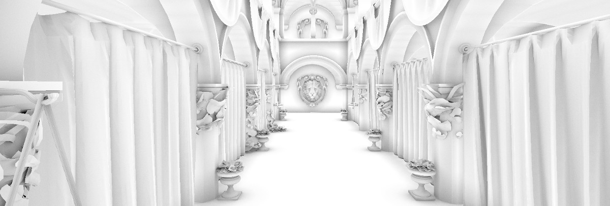
End result. Sponza scene with basic Phong lightning.
Top is the scene composed with the ambient occlusion we're going to compute.
The temporal accumulation is reset while moving, creating a noisy output for a few frames.
Future articles:
- Shadows and denoising (filtering, clever temporal accumulation)
- Translucency
- Hybrid rendering (combining rasterization and ray-tracing)
Starting from somewhere
I'm currently working on a game engine called lava. I had implemented a standard rasterizer that just does simple rendering, with no tricky effects. But when you want to get really fancy, good lighting and such, in rasterizers that's getting hard to implement.
Before going into the details of the ray-tracing stuff, let's recall what's a rasterizer.
Classic rasterization
A rasterizer is a 2D thingyfier, it understands basically nothing apart from 2D triangles.
Wait… 2D? But our games are 3D, right?
Well… your meshes might be 3D, defined with 3D points (x,y,z) and 3D normals and such.
 All complex meshes are made of simple primitives, usually triangles.
But we're talking about the renderer. And my point is that a rasterizer will basically just process this:
 A bunch of 2D triangles.
Here points are defined with 2D coordinates (x,y), relative to the image space.
We use a projection matrix to project the 3D points into the 2D world of the graphic card. Every vertex shader begins with this projection.
And we use a well-known trick (depth buffer) to correctly display front triangles above those below. This classic technique is integrated into graphic APIs, and graphic card vendors have specialized hardware to make it fast.
Lighting is then done with math. We compute an imaginary ray from a light and, using mystic material-dependent parameters, we make our objects look realistic.
Translucent materials are more challenging than opaque ones and require more tricks to work. I tried integrating them more naturally, but they broke our previous depth buffer trick. Now, we're stacking tricks to make things work.
There are even more dedicated algorithms to achieve good-looking results. A lot of tricks again. They all involve clever, specific code and architecture, such as motion blur, bloom, subsurface scattering, iridescence, depth of field, and - the one discussed in this article - ambient occlusion.
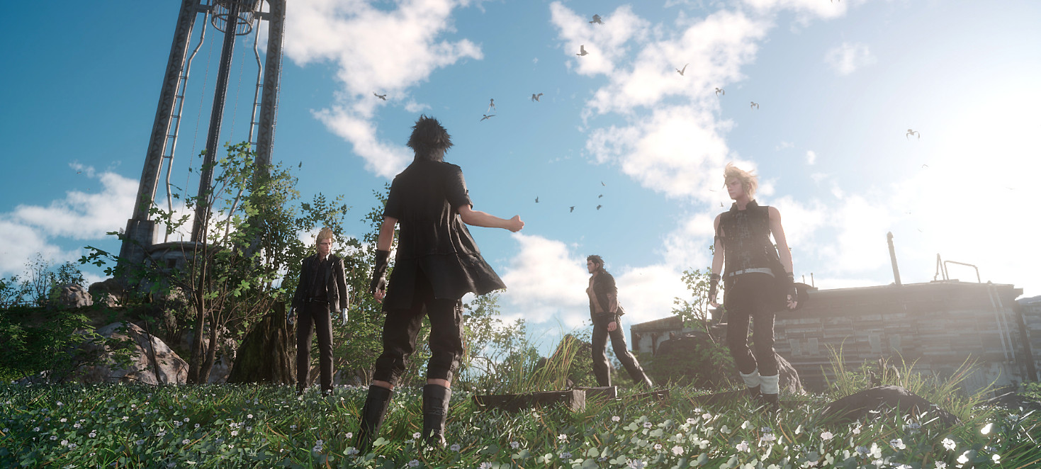 So many tricks to get a good looking image.
Source: Final Fantasy XV - © Square Enix
Tricky ambient occlusion
Ambient occlusion (AO) shadows objects in proximity. It does not replace projected shadows caused by obscured light sources; instead, it shows when light reflection struggles to pass through small spaces.
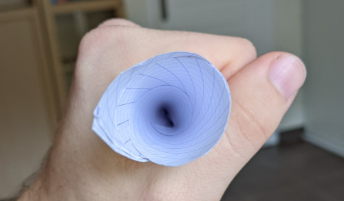 Look at what I made! A paper cone.
Ambient light is entering the cone, but the deeper we go, the less light can get out.
I guess I could have shown the classical image of walls, where the corners are darker than the panes, but I wanted to show my crafting skills.
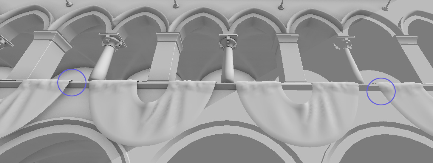 In rendering engines, enabling AO adds a lot. This is a scene with and without AO.
Very close triangles occlude each other and add realism.
In rasterizers, AO falls into two categories:
- Precomputed: for static geometries, whenever possible.
- For instance, the glTF format for 3D models allows the use of an
occlusiontexture. This texture is usually computed with the 3D software of the artist.
- For instance, the glTF format for 3D models allows the use of an
- Real-time: for when the user has a powerful machine.
- SSAO (Screen-Space Ambient Occlusion) is a now common post-processing technique that uses sophisticated calculations to achieve its effect. It uses the normal and depth of each final pixel rendered.
- HBAO (Horizon-Based Ambient Occlusion) is an improved SSAO trying to achieve more physically-based results. NVidia presented it in SIGGRAPH 2008 better than I would be able to.
In one word, real-time AO in rasterizers is hard-and-imprecise. This is mainly due to the fact that meshes are treated separately, and the graphic card only knows one geometry at a time. Therefore, the best you can do is to post-process the image and crossing your fingers for not too much artifacts. (Pro-tip: never really cross your fingers while coding.)
So, this was a somewhat complicated introduction, wasn't it? Well… that's the point: rasterizers are remarkably complex. As the next section will detail, ray-tracers are suprisingly intuitive.
Going somewhere new
Ray-tracing, briefly
Ray-tracing is about launching rays in a 3D world. Here we go, I said it: ray-tracing is 3D, while rasterizing is 2D. For real-time ray-tracing, GPU will then need the whole world you want to render at one time.
Once the GPU has everything, we tell it to launch a ray from an origin in a certain direction, and we will be called each time that ray hits our geometry.
 Taken from "Reflections", a real-time ray-tracing demo in 2019. - © NVIDIA
Vulkan 1.2 has a dedicated terminology for handling ray-tracing in its API, and that's the one I'm going to use below. I believe that Direct3D has the same words, but I'm not an expert, so maybe there are some differences.
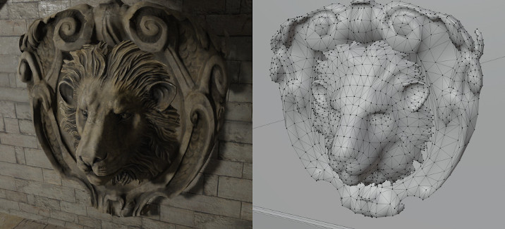
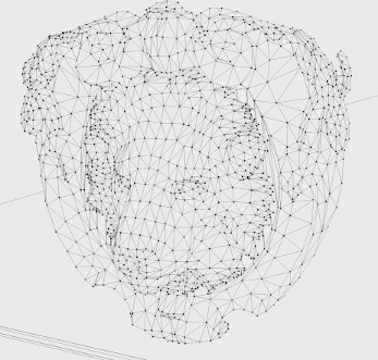
The 3D geometry is baked into acceleration structures, which are probably implemented with bounding volume hierarchies (BVH) by vendors.
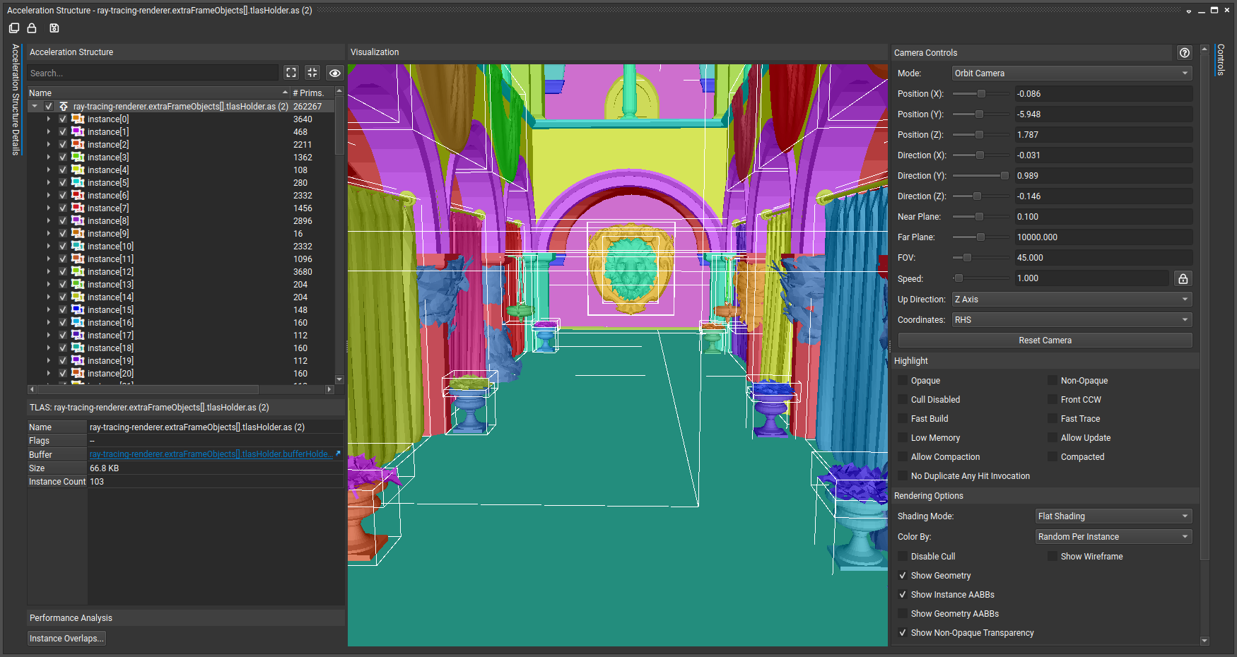 Our acceleration structures shown within NVIDIA Nsight Graphics.
Each bottom-level acceleration structure instance gets its own color and the bounding boxes are displayed.
Then, we use a RayGen shader to launch our rays and let the GPU resolve the ray-vs-geometry intersections.
When a hit occurs, an AnyHit shader is triggered, and when the traversal is finished, we either get a ClosestHit or a Miss shader called.
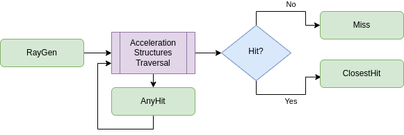 Ray-tracing pipeline.
(Intentionally not talking about the Intersection shader here, even though it's a great feature.)
What's fun is that all these shaders can relaunch rays. This makes the whole thing exponentially costly, but really powerful.
That's great, let's do AO, then!
Almost real-time ray-traced AO
Make it slow and look good
As always, a drawing is often easier to understand:
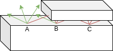 The basic idea to compute AO.
For each pixel that need to be rendered, launch a bunch of rays and compute how many do not intersect something.
Shadow the pixel based on this value.
Technically, we would need a infinite number of rays per pixel to compute the hemispheric region intersections. So, instead, we will use let say 1000 random rays per pixel and compute the percentage of intersecting rays. And if you want to search literature on the subject: this is called a Monte Carlo integration.
And an important point to make is that these rays are not of infinite length. Otherwise the roof could occlude the floor. I'll just say that above 0.5 meters, we don't occlude. But we'll tweak this parameter later on.
0.01m or 0.49m will have the same impact.There are two reasons behind that choice. First, we are launching a lot of rays, so the mean will reflect a more sensible result than one ray intersection. Secondly, the
TerminateOnFirstHit optimization I'll describe a bit below would not be possible.
Let's sum up all that in a small pseudo-code.
# RayGen
- For each pixel:
     - payload.intersections := 0
     - For rayIndex := 1..1000:
          - ray := a random ray around the hemisphere directed by the surface's normal
          - launch 'ray' with a max length of 0.5
     - aoOutput := 1 - payload.intersections / 1000

# ClosestHit
- payload.intersections += 1
First try of a pseudo-code for AO.
We have already a lot to discuss here.
We're using a ClosestHit shader because a AnyHit shader would be called for every intersection along the ray path, hence potentially counting too many intersections.
What's payload? It's the secret behind communication between ray-tracing shaders. RayGen and ClosestHit are different programs but they will share a memory area called payload. And I'm a bit lying about the For each pixel being within the RayGen shader. It's not the case, in fact, we have multiple RayGen shaders running at the same, one for each pixel. Each of those has its own payload memory.
The aoOutput := 1 - (whatever) part is due to 1 meaning white and 0 meaning black in graphics programming. Therefore, we reverse the output so that shadowed areas are black. You can see that if all intersections are detected, the output is black. In fact, if we switch the logic, the algorithm becomes a bit cleaner:
# RayGen
- For each pixel:
     - payload.misses := 0
     - For rayIndex := 1..1000:
          - ray := a random ray around the hemisphere directed by the surface's normal
          - launch 'ray' with a max length of 0.5
     - aoOutput := payload.misses / 1000

# Miss
- payload.misses += 1
Second iteration of a pseudo-code for AO.
By switching from a ClosestHit shader to a Miss shader, the AO is slightly easier to compute. And, more importantly, we enabled an optimization.
traceRayEXT(topLevelAccelerationStructure,
            gl_RayFlagsTerminateOnFirstHitEXT | gl_RayFlagsSkipClosestHitShaderEXT,
            /* ... */
);
Flags in shader code optimizing the launch of AO rays (GLSL).
We're allowed to say "don't run the ClosestHit shader", but not for the Miss one. By using these flags, we're able to save a lot of computations.
I somehow wrote the sentence "a random ray around the hemisphere directed by the surface's normal" with a straight face. But there are three points to tackle hidden in it.
- random: how do we get a random number in a shader?
- around the hemisphere: how do we take a sample of an hemisphere?
- directed by the surface's normal: how do we make the normal be the main direction?
Randomness in shaders
One good thing about randomness in shaders is that you often find yourself not really wanting pure randomness. You want just something that looks random. Fact is blue noise is considered to be giving better results than classical white noise in our domain. But I will not tackle that in this article. Feel free to document yourself, I just want a working example without too many layers to understand. (I might go back to this subject in future articles though.)
I won't lie, I've just stolen some code:
uint hash(uint x) {
    x += (x << 10); x ^= (x >> 6);
    x += (x << 3);  x ^= (x >> 11);
    x += (x << 15);
    return x;
}

float floatConstruct(uint m) {
    const uint ieeeMantissa = 0x007FFFFF; // binary32 mantissa bit-mask
    const uint ieeeOne      = 0x3F800000; // 1.0 in IEEE binary32

    m &= ieeeMantissa;    // Keep only mantissa bits (fractional part)
    m |= ieeeOne;         // Add fractional part to 1.0

    float  f = uintBitsToFloat(m);  // Range [1:2]
    return f - 1.0;                 // Range [0:1]
}

float random(float x) { return floatConstruct(hash(floatBitsToUint(x))); }
[0:1] random numbers generator, as proposed by user Spatial on StackOverflow (GLSL).
The idea is simple, yet very efficient: use a classical hashing function on integers and build a float from its output.
And by XORing two hashes on the pixel (x,y) position in the image and one hash from the ray index we want to the launch, we get a random number for each ray we want to launch.
 White noise generated with Spatial's algorithm.
Cosine-weighted sampling
We've got some flat random numbers, but we want a random point on the hemisphere directed by the up vector (0,0,1). Hidden in some mathematical details greatly explained in Ray Tracing Gems I on page 211, our Monte Carlo estimator require a cosine-weighted sampling.
// Where x0 and x1 are uniformly distributed random numbers in [0, 1].
vec3 sampleZOrientedHemisphericDirection(float x0, float x1) {
    return vec3(sqrt(x0) * cos(2 * PI * x1),
                sqrt(x0) * sin(2 * PI * x1),
                1 - sqrt(x0));
}
Magic (GLSL).
To be honest, I am really not comfortable explaining all this, because I don't understand much. So I'm just going to test it.
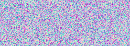 Output of one sampling per pixel, where unit vectors have been remapped like a normal map.
It's mostly blue, so it means it mostly goes into the (0,0,1) direction. Let's say I am OK with this sampling, then.
Transform to surface's normal
This part is no more statistics, so I feel better. It's linear algebra.
So we have a hemisphere directed by (0,0,1) and we want move it into the direction of the surface's normal (nx,ny,nz).
Here's what I did:
mat3 makeRotationMatrix(float angle, vec3 axis) {
    float c = cos(angle);
    float s = sin(angle);
    float t = 1.0 - c;
    vec3 tAxis = normalize(axis);
    return mat3(
        tAxis.x * tAxis.x * t + c,
        tAxis.x * tAxis.y * t - tAxis.z * s,
        tAxis.x * tAxis.z * t + tAxis.y * s,
        tAxis.x * tAxis.y * t + tAxis.z * s,
        tAxis.y * tAxis.y * t + c,
        tAxis.y * tAxis.z * t - tAxis.x * s,
        tAxis.x * tAxis.z * t - tAxis.y * s,
        tAxis.y * tAxis.z * t + tAxis.x * s,
        tAxis.z * tAxis.z * t + c
    );
}

mat3 reorientZOrientedDirectionMatrix(vec3 targetDir) {
    if (targetDir.x == 0 && targetDir.y == 0 && targetDir.z == 1) {
        return mat3(1, 0, 0, 0, 1, 0, 0, 0, 1);
    } else if (targetDir.x == 0 && targetDir.y == 0 && targetDir.z == -1) {
        return mat3(1, 0, 0, 0, 1, 0, 0, 0, -1);
    }

    float angle = acos(dot(targetDir, vec3(0, 0, 1)));
    vec3 axis = cross(targetDir, vec3(0, 0, 1));
    return makeRotationMatrix(angle, axis);
}
Creating a rotation matrix that goes from the up vector to a direction direction.
There was probably some clever trick based on quaternions (mostly because a quaternion is just an axis and an angle slightly altered), but I'm just happy with that.
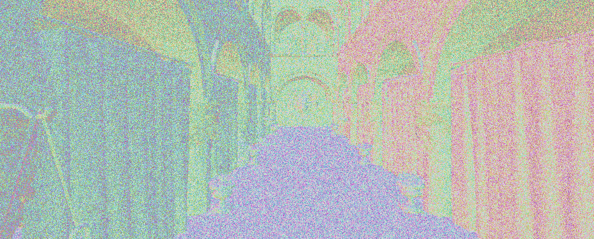 Entering the matrix. Visualizing one random ray per pixel directed by the surface's normal.
We're almost done. Now that we can generate random rays correctly, we're just back to the original algorithm: check if they collide and take the mean of them all.
Shuffling all that together
Let everything run and…
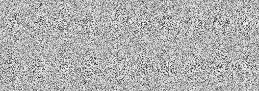
 The pure AO output at 1000 rays/pixel with 0.5 ray length.
Yeah! Looks clean, right? Let's tweak some parameters just to see their impact…
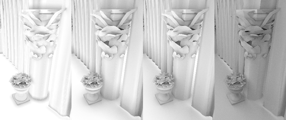 With 0.1, 0.5, 1 and 5 ray length.
Small ray length results in very peculiar AO, where the shadowed areas are very concentrated. With the increase of that parameter, AO gets darker and noisier. The noise is because our hemisphere's border is larger and we need more rays to approximate it better. The darkness is due to very far things still occluding each pixel.
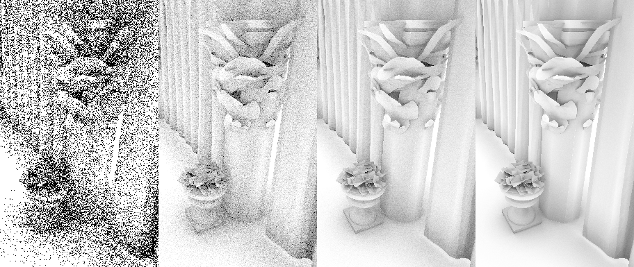 With 1, 10, 100 and 1000 rays/pixel.
The AO gets smoother and smoother with the increased number of rays, as we get a better approximation of the hemisphere. The noise in 1 or 10 rays/pixel is very invasive.
To sum up, our choice of 1000 rays/pixels with a ray length of 0.5 was sensible for a good looking result. However, there's one more thing to check…
| 1 ray/pixel | 10 rays/pixel | 100 rays/pixel | 1000 rays/pixel |
|---|---|---|---|
| 1.67ms | 6.03ms | 49.38ms | 485.1ms |
These results are for generating one 1600x900 frame on a RTX 3070. It definitely depends on the complexity of the scene also, but there's one takeaway: it's either slow or ugly. Let's keep the fast one and make it look nice.
Real real-time ray-traced AO
Make it slow and look good
This series of article is entitled "Ray-tracing in 10ms", and I will want to make other effects. So the best I can spend is 1 ray/pixel. Not even two.
There are two paths to clean the output of 1 ray/pixel/frame.
- Filter via a denoiser pass. But I'll talk about that in the article on shadows.
- Accumulate on multiple frames by not forgetting previous results.
I'm going to explain how I made a stupid temporal accumulation. But in a real product you probably want a combination of both methods.
So far, we've been doing:

where the mean is equal to the sum of n = 1000 rays intersection results divided by 1000. I want to switch perspective and just do 1 ray/frame, storing a iterative mean and updating it. With some math tweaking we get:

By making the mean iterative with this formula, we can compute the mean at frame f + 1 based on the mean computed at frame f.
And that's all, we can just store a previous frame AO and update it each time. If we have accumulated more that 1000 rays, we stop computing the AO because the impact of the new values would be minimal.
The one thing I add that I reset the accumulation whenever the camera moves, so that the stored result is only valid for non-moving points.
Here we go, then:
Go full-screen and have a look on dark areas, you'll see the temporal accumulation.
Frame count is displayed in the bottom of the screen.
What's next
The intro video of the article shows what happens when moving the camera. It is also AO composed with a basic Phong lighting.
One can notice artifacts like very black dots in the top part of the screen, these are due to the precision of floating point operations and the complex geometry. They will eventually go away with denoising.
Finally, you can find the code of these shaders on my engine's repository under the MIT license. Feel free to get inspired by those.
See you "soon".
Great references and tools in random order
- Ray Tracing Gems series
- Sascha Willems' Vulkan repository examples on GitHub
- NVIDIA's Vulkan ray-tracing tutorial
- Khronos' Vulkan 1.2 specification explanation
- RenderDoc (no ray-tracing support at the time of this article, sadly)
- NVIDIA NSight Graphics (with ray-tracing support, nicely)
- The commit associated with AO implementation within my engine